Copying a Worksheet into another Workbook

How to make a copy of a Worksheet from the current Workbook to another Workbook?

1. Open the Target Workbook, when the Source Workbook is already in open state.
2. Right-Click on the Source-Worksheet Tab.
   
3. Select the Move or Copy... option from displayed shortcut menu.
4. Select the Target Workbook name from the To Book: drop-down list.
   

5. Put a check-mark in the Create a Copy option and click OK.

There you are, you have a clone of the source worksheet on your Target Workbook.

Instead, if you want to move a worksheet to the target Workbook, select (Move to End) option.

Read More

Data Validation in Excel

Excel Worksheet Cell accepts values of any data type viz. Text, Number, Date/Time or expressions (result values can be any of these types).  Worksheets are the best tools for What…If analysis and present numerical data in Graph Chart form.  Besides all these we can create databases on worksheets and query information very quickly.

An Excel Database is like any other worksheet but created with few basic rules of databases in mind so that certain querying operations can be performed, like searching, filtering, lookup and so on.  I will list few basic rules, that you should know about setting up an excel based database (table) structure, below.

1. The topmost row columns of a table should have the data Field Names and all of them should be unique (no duplicates) and cannot be in merged cells. 
2. There should not be any column without column heading within the table area.
3. Data type of each column should be of same type, like text or Number or Date or a formula that results in the same data type, not the mix of different data types in the same column.
4. There should not be any blank rows within the table range, but some cells in a row can be empty, if needed.

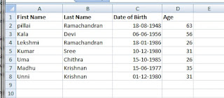
These are some of the simple rules that goes for defining an excel based database. Image of a sample database is given below:

There are several built-in database functions in excel, like DSUM(), DAVERAGE(), DCOUNT() and others for analysis purposes, but the data must be reliable.  We have to ensure that the data entered into the data fields keep up with the strict rules that we set for each field.

A single cell under the First Name field can accommodate thousands of characters. We don’t need that much text in the First Name field.  But, we must be able to enter enough text (say a maximum of 25 characters) in the First Name field and about that much in the Last Name field as well, not more than that.

A list of validation rules applicable for each data field is given below. We will use these rules to perform validation checks on keyed-in data (result of expressions are not validated) before they are being accepted into the data field.

Data Validation Rules

Serial	Field Name	Data Type	Length	Validation Rule
1.	First Name	Text	25	Text Data, maximum length 25 characters
2.	Last Name	Text	25	Text Data, maximum length 25 characters
3.	Date Of Birth	Date		Future Date and Date earlier than 100 Years not Valid
4.	Age	Number		Range 1 - 100

Now, let us try to implement the above rules in an excel Table area and experiment with it to see how these rules actually works while entering data into each column.

1. Open a blank Excel Workbook.
2. Enter the Table headings in Range A1 to D1 as shown in the image given above.
3. Select the first cell below the column heading First Name.
4. Select Data Validation . . . from the Data Tools Toolbar buttons group under the Data Menu. The Validation settings dialog control opens up like the image shown below:
   
5. Select the Settings Tab.
6. Select Text Length from the Allow: control’s drop-down list.
7. Select Less than or equal to from the Data: control’s drop-down list.
8. Type 25 into the Maximum control. The cell with this settings will allow only 25 characters of input into the cell.
9. Select the Input Message control.
   

   When the User selects the Cell to key in data the settings on the Input Message control will appear as a comment box attached to the cell, to guide the user to enter a valid value, or with whatever message you intended to convey.

10. Put check mark in the ‘Show input message when cell is selected’ control.  If check mark is not present then the message we set up in the next two steps will not appear on the worksheet.
11. Type First Name in the Title control.
12. Type Enter First Name (25 characters)  in the Input Message control.
13. Select Error Alert Tab.  This is where we have to set up the real validation check to perform and alert the user when invalid data is entered into the cell.
    
14. Put a check mark in the ‘Show Error Alert after invalid data is entered’. If this is not enabled then the user will not be warned on entry of invalid data.
15. Select the Icon style (Stop, Warning or Information) of Alert message box, default stop will be just fine.
16. Type First Name in the Title control.
17. Type Maximum 25 characters.
18. Click OK to close the dialog box.
19. Select the first cell below Last Name field.
20. Repeat Step-4 to Step-18 replacing First Name field name with Last Name, wherever applicable.
21. Select the Cell beneath the Date Of Birth field.

    We will prevent this field from accepting a future date for Date of Birth.

22. Select Data Validation option to open up the dialog control.
23. Select Date from the drop-down list in the Allow: control.
24. Select Less than or equal to in the Data: control.
25. Type =TODAY() in the End Date: control.

    As you can see we can enter a Function or expression in this control rather than a constant value, when needed.

26. Select the cell below the Age field.
27. Enter the following expression to calculate the Age, based on the Date of Birth field value:

    >=INT(IF(C2>0,(TODAY()-C2)/365.25,0))

    We will leave this field from validation checks.  Validation checks can be performed only on cells where manual keying of data is done. 

28. Highlight Cell Range A2:D2 and Right-Click on the highlighted range.
29. Select Copy from the shortcut menu.
30. Highlight Range A3:A20 Right-Click on the highlighted range.
31. Select Paste Special from the shortcut menu.
32. Select the Radio Button with the label Validation under the Paste options and click the OK button to apply the Validation rules we have copied from the source range A2:D2 into the target area A3:D20.
33. Highlight Cell D2, right-click and select Copy from the shortcut menu to copy the Formula from cell D2.
34. Highlight Range  D3:D20, right-click and select paste from the short-cut menu.

    Tip:  You may press Ctrl+C to copy the source cell and press Ctrl+V to paste the formula after highlighting the cell ranges.

35. Save the Workbook file with a name.

Now, let us test our database’s validation checks.

1. Type a name with more than 25 characters in length into Cell A2.  When the Error Alert pops up click Cancel and enter a name with 25 characters or less.
2. Type something similar in Cell B2 with more than 25 characters.
3. Type tomorrow’s date into Cell C2.

Key Words:Validation,Input Message,Error Alert

• Welcome Message in Application
• Welcome/Good-Bye Messages
• Displaying worksheet Formula

Read More

Display 12 Months Charts in one Chart Object

I know, we need some details on this to start with.  Since, this is all about Graph Charts I will present some data for our chart below then go into details about the whole project.  Here is the image of sample Chart prepared using the sample data shown above the Chart:

The sample data is the summary of Revenue, Expenses detail statements located elsewhere on the Worksheet and not shown. The statement includes data of three Branch locations of a Company for the month of January.

When Graph Charts are prepared this way, our Workbook will have twelve Worksheets and twelve Graph Charts for the months from January to December.

When your Boss wants to review the Summary Data/Graph Chart of any month he has to select the Worksheet of that particular month to view the data or Graph Chart.  He/She has to move from one worksheet to the other to view the information/chart from different worksheets.

But, with a cool trick we can make this task very easy and show the Summary statement of any month and it's corresponding Graph Chart on particular location on a worksheet, based on the month selected from a Listbox. Besides that you don't need to prepare Graph Charts on all twelve month's Worksheets. But the Summary data must be present on the same Range location on all twelve worksheets, for JAN to DEC.

For example, the summary statement shown for the month of January in the above image is placed within the Cell Range L10:O13 on JAN worksheet. The actual Revenue, Expenses and Profit/Loss Values are within the Cell Range M11:O13. Summary statement of all twelve months must be maintained on the same Range Address on all Worksheets of JAN to DEC.

Image of our Planned Worksheet is given below:

Check the Worksheet Tabs at the bottom of the image, you will find that we have added two more Worksheets with the name 'Control' and 'Ctrl_data' besides worksheets of JAN to JUN. The Control Worksheet holds sample Summary data in Range A1:D4. The Graph Chart shown there is prepared from the sample data. The Listbox at the left side of the Chart holds the names of the month, or the Worksheet names that holds the summary data for the month of JAN to DEC. When the user selects a month (say MAR) from the listbox a Macro connected to the Listbox runs and copies the summary data from the selected Worksheet Summary data Range: M11:O13 and paste it into the Control Worksheet sample summary data area: A1:D4. The Graph Chart automatically reflects the change immediately. The user can select any month of his choice from the list and its corresponding data will be brought in to the Control worksheet and the Graph will change accordingly. So your Boss can stay on the Control worksheet and view the Summary Statement and Graph Charts of any month selected by him/her from the Listbox.

Now, let us get to work to build our trick. We assume that you have Excel2007, while referring to Menus and Options.

1. Open a new Workbook and save it with a name and in Macro enabled format (with .xlsm Extension). If you are using Excel2003 then you may save it as you do normally.
2. Right-click on Sheet1 and select Rename from the Shortcut Menu and change the name of the worksheet as JAN.
3. Rename the other two Worksheets as FEB and MAR.
4. Select JAN worksheet and create sample Graph Chart data, as shown on the first image above, and within the same Cell Range: L10:O13 .   Don’t create any Graph Chart there.
5. Copy the data from JAN worksheet and Paste it on FEB and MAR worksheets on the same Cell Range.  Make some changes in Revenue, Expenses figures on FEB and MAR worksheets.  Profit/Loss Value is the difference between Revenue and Expenses.

   Now, we need two more Worksheets.

6. Insert a new worksheet and rename it as Ctrl_Data.
7. Type the information on the Ctrl_Data worksheet as shown in the image below. 

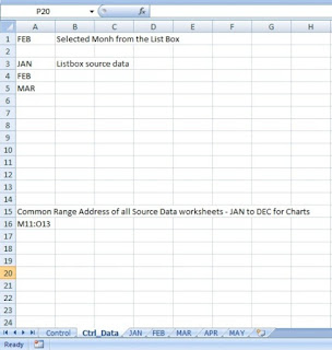
We need to create one more Worksheet with the name Control. The worksheet image is the second one from top.  Before going into that let us check the Ctrl_Data worksheet contents.

• Cell A1 holds the value selected from the Listbox and it is for System use only.
• Cell Range A3:A5 holds the source data for the Listbox.  This can be expanded up to the month DEC, when you add more sheets to your workbook.
• Cell A16 holds the common Range Address of JAN to DEC worksheets, where the Revenue, Expenses & Profit/Loss Values are stored.

1. Insert a new worksheet and rename it as Control.
2. Copy the sample data from Range L10:O13 of JAN worksheet and paste it in Cell A1 on Control worksheet.
3. Click on the Insert drop-down control in the Controls group under Developer Menu.
4. Click the Listbox Tool to select it from the ActiveX Controls group, rather than from the Form Controls group.
5. Draw a Listbox somewhere below the sample data on the Control worksheet.  Check the Listbox shape on sample Control worksheet image above (second from top).
6. While the Listbox is in selected state click on the Properties button in the Controls group under the Developer Menu.  Check the Control worksheet image below with the Listbox’s Properties Sheet displayed.
   

   We will be making changes to four different property values on the Property Sheet.

7. Check the Name Property Value, if it is not set as ListBox1 then change it to read as ListBox1.
8. Locate the Property LinkedCell and type: Ctrl_Data!A1 at the right column.
9. Type: Ctrl_Data!A3:A14 for the ListFillRange property.  When you update this property you can see the Listbox control is filled with the month names: JAN, FEB & MAR.
10. Check whether the MultiSelect Property is set with the value: 0 – frmMultiSelectSingle or not, if not then set it as 0 – frmMultiSelectSingle from the Drop-down box.
11. Click on the Close (X) button (top right corner of the property sheet) to close the property sheet.
12. While the Listbox is still in selected state, click on the View Code button, near the Properties button, to open the VBA Code Window with the empty ListBox1_Click()  Event Procedure’s starting and ending lines.
13. Copy and paste the Macro Code given below over-writing the existing ListBox1_Click() Event Procedure:

    Microsoft Excel2007 Version Code:

    Private Sub ListBox1_Click()
    Dim m_mth, m_Range
    On Error GoTo ListBox1_Click_Err
    m_mth = Worksheets("Ctrl_Data").Range("A1").Value
    m_Range = Worksheets("Ctrl_Data").Range("A16").Value
    'if clicked on an empty area in the list box, then exit
    If Len(m_mth) = 0 Then
      Exit Sub
    End If
    'Insert selected month Name in the Chart Data area left corner cell
    Worksheets("Control").Range("A1").Value = m_mth
    'Copy the cell Source Range contents
    Sheets(m_mth).Range(m_Range).Copy
    Sheets("Control").Activate
       'Paste copied values into the Control Worksheet Range
       'Starting with Cell B2
       ActiveSheet.Range("B2").Select
        Selection.PasteSpecial Paste:=xlPasteValues, Operation:=xlNone, SkipBlanks:=False, Transpose:=False
      'Set reference to the Chart Object on Control Worksheet
      With Worksheets("Control").ChartObjects(1).Chart
        .HasTitle = True
        .ChartTitle.Text = "Profit/Loss - " & m_mth & "/" & Year(Now())
      End With
    ListBox1_Click_Exit:
    Exit Sub
    ListBox1_Click_Err:
    MsgBox Err.Description, , "ListBox1_Click()"
    Resume ListBox1_Click_Exit
    End Sub

    Microsoft Excel97-2003 Code:

    Private Sub ListBox1_Click()
    '---------------------------------------------------------
    'Author : a.p.r.pillai
    'Date   : May 2012
    'Remarks: All Right(c) Reserved by excel.msaccesstips.com
    '---------------------------------------------------------
    Dim m_mth, m_Range
    On Error GoTo ListBox1_Click_Err
    m_mth = Worksheets("Ctrl_Data").Range("A1").Value
    m_Range = Worksheets("Ctrl_Data").Range("A16").Value
    'if clicked on an empty area in the list box, then exit
    If Len(m_mth) = 0 Then
      Exit Sub
    End If
    'Insert selected month Name in the Chart Data area left corner cell
    Worksheets("Control").Range("A1").Value = m_mth
    'Copy the Source Cell Range contents
    Application.CutCopyMode = False
    Sheets(m_mth).Range(m_Range).Copy
    Sheets("Control").Activate
    'Paste copied values into the Control Worksheet Range
    'Starting with Cell B2
       ActiveSheet.Range("B2").Select
       ActiveSheet.PasteSpecial Format:="Text", Link:=False, DisplayAsIcon:=False
      'Set reference to the Chart Object on Control Worksheet
      With Worksheets("Control").ChartObjects(1).Chart
        .HasTitle = True
        .ChartTitle.Text = "Profit/Loss - " & m_mth & "/" & Year(Now())
      End With
    ListBox1_Click_Exit:
    Exit Sub
    ListBox1_Click_Err:
    MsgBox Err.Description, , "ListBox1_Click()"
    Resume ListBox1_Click_Exit
    End Sub

    Now we must create the Graph Chart using the sample data on the Control worksheet.

14. Highlight Cell Range A1:D4.
15. Click on the Column drop-down control, from the Charts group of Insert Menu, and select the first Column chart type.
16. Draw a Graph Chart, like the sample Chart shown on the second image on the top, at the right side of the Listbox. 
17. If Chart Title is not shown on the top area of the Graph Chart then select the first Chart Layouts option under Design Menu.
18. Right-click on the first Data Series Bar.
19. Select the Add Data Labels option from the displayed Shortcut Menu.
20. Set data labels for the other two set of Bars too.
21. Save the Workbook.
22. Select the Developer Menu and click on the Design Mode button to de-select it.

Now, it is time to try out our Project.

Click on FEB in the Listbox control.  If everything about the design tasks went through well then you should see the Graph Chart Data is copied from the FEB worksheet to the Control worksheet summary data Range: B2:D4 and the Graph chart displays information for the month of February.  The Graph Chart Title also changes automatically.

Click on JAN or MAR in the Listbox and watch the selected month’s summary data and Graph Chart appears on the Control Worksheet.

Tip:  You may add worksheets for APR to DEC with sample data and update the Listbox contents on the Ctrl_Data worksheet to try out the program for all twelve months.

• Welcome/Good-Bye Messages
• Displaying worksheet Formula
• Microsoft Excel Automation

Read More

Welcome Message in Application

Let us try a small trick with VBA.  How about a welcome message pops up automatically when you open your Excel Workbook and a Goodbye message before closing the Workbook?

We assume that you are using Microsoft Excel 2007.

1. Open one of your existing Excel Workbooks or create a new Workbook to try this out.
2. Click on the Visual Basic option under Developer Menu to open the VBA Module Window.
3. Check the VBA Window image given below.

The VBA Window is divided into two parts.  The top window area shows the list of Worksheets and other objects in the active Workbook.  The Code area below is where we can write Code to automate certain actions so that working with the Excel Application becomes easy to the Users and interesting too.  You can see one line default code Option Explicit (says needs to define variables before they are referenced in programs) is appearing in the code window area.

If you look closely on the top window area you can see that Sheet1 (mySheet) Object is in selected state.  The name in bracket (mySheet) is appearing because I renamed Sheet1 as such.

1. Click on the drop-down control, where the text (General) is shown, to display the Object type selected in the above window.
2. Select Worksheet from the displayed list. You can see an empty skeleton of Worksheet_SelectionChange() Sub-Routine is added as default to the VBA Editing window. But, we don’t need that for now.
3. Click on the right side drop-down control to display the available event procedure’s list, which can be selected and programmed on the worksheet object to automate worksheet related actions.  We are not going to write any code within the default program block added into the VBA editing window.  You may delete the opening and end statements of the procedure of Worksheet_SelectionChange() Sub-Routine.
4. Now, click on the ThisWorkbook object from the Window above to select it.
5. Select Workbook in the (General) Control from the drop down control.

The opening and closing statements of the Open Event Procedure of the Workbook is added to the VBA Editing window as default.  You can see that the action type Open is selected as default in the right side drop-down control.  Whatever action code we write within the Workbook_Open() Event Procedure will be executed automatically and immediately on opening the Workbook.  We will write a single line of code to display a welcome message when the workbook is open.  Modify the code as shown below by adding the middle line with the MsgBox() Function.

Private Sub Workbook_Open()
    MsgBox "Welcome to Excel Application", vbInformation + vbOKOnly, "Workbook_Open()"
End Sub

The MsgBox() Function needs at least the first parameter value i.e. the Message Text, second and third parameter values are optional.

Second Parameter value is a combination of three different values, but any of them or all of them can be omitted in MsgBox() function:

• Specifies the type of Message box icon type, like information, question, help and so on.
• Message Box Buttons, like OK button only or OK and Cancel buttons or Abort, Ignore and Retry buttons etc.
• Third item specifies which button is selected as default, if more than one button is specified.

Example for second parameter:

MsgBox "Logical Errors in Program",vbAbortRetryIgnore+vbCritical+vbDefaultButton2,"Main()"

The highlighted values can be in any order joined with + sign.  The highlighted text is actually VBA defined Integer Constant values and they are added up together and the result value is used for displaying the message box Icon and Buttons.

Image of the Message Box displayed with the above statement is given below:

• vbAbortRetryIgnore - specifies the message box should have Abort, Retry and Ignore Buttons and it is defined as a VBA constant like Public Const vbAbortRetryIgnore As Integer = 2.
• vbCritical - specifies the message box icon. vbCritical = 16.
• vbDefaultButton2 - says select the second option (Retry button) as default. vbDefaultButton2 = 256.
• vbAbortRetryIgnore+vbCritical+vbDefaultButton2 = 2+16+256.

The above values can be specified in any order and is optional.  If you omit the second parameter the OK Button will appear in the Message Box.

Third parameter is the Title Text (appears on the top) of the message box and is optional.  Normally it carries the name of the Function or Sub-Routine, if specified.  If the message box is used for reporting logical errors the title can give the programmer a clue as where to look for debugging the code.

Before trying out the above Open Event Procedure we will add one more message box to display a message before closing the active workbook.

1. While the Workbook object is in selected state in the left side control select BeforeClode from the right side drop down list.
2. Modify the new procedure with the following lines of Code or copy and paste it:

Private Sub Workbook_BeforeClose(Cancel As Boolean)
Dim txtMsg As String
Dim buttons As Integer
txtMsg = "Shutting Down Excel Application, Bye."
buttons = vbInformation
MsgBox txtMsg, buttons, "BeforeClose()"
End Sub

1. Save the Workbook in Macro Enabled Format (with .xlsm extension) and close it.  If your workbook is not in macro enabled format (Excel2007) then Excel will prompt you to save the workbook in a Macro enabled format (with .xlsm extension). If you don't select this format you will loose the program you have written in your Wokbook.
2. Open the Workbook with our programs.  You will see the Welcome message from the first program, immediately after opening the Workbook.
3. Now, close the Workbook.  Before closing the Workbook the BeforeClose() program runs and displays the “Shutting Down Excel Application, Bye.” message.

• Displaying worksheet Formula
• Microsoft Excel Automation
• Microsoft Excel Automation-2

Read More

Displaying Worksheet Formula

Worksheets can have hundreds of  formulas linked to one another.  Output value of one cell formula can become part of another formula in another cell.  When worksheets of this type involves in complex analysis tasks it becomes difficult to track the relationships between formulas in cells or range of cells, especially when cell references depends on Cell Addresses.  When you insert cells, rows or columns the cell references in formulas can change.

When you start developing something  serious it is a good idea to give unique range-names to Cell or Range of Cells and use those names in expressions.

For example:

Assume that Cell Range B2:B25 contains detailed figures of Income values.  This Range of Cells can be easily referenced with the Range Name Income.  Try the following:

1. Open Microsoft Excel and fill some numeric values in Cells B2 to B25 on Sheet1.
2. Highlight the Cell Range B2:B25.
3. Select Define Name from the Defined Names group from Formulas Menu and type Income as name into the Name control in the displayed dialog box.  The selected Range address will be displayed in the Refers To: control at the bottom of the dialog box as =Sheet1!$B$2:$B$25.
4. Click OK to return to the Worksheet.
5. Select Cell B26 and Type the expression =Sum(Income) to get the sum of values from Range: B2:B25.

   Note: If you add few rows/cells between B2:B25 and  add values into the added Cells, the Income range will automatically expanded and the correct value will reflect in wherever we use the Income range name.  If you add rows or cells above Cell B2 the Income range will automatically adjust itself to refer to the number of cells within the Income Range to the changed position.

   For example: if you have added a single row above the cell B2, the Income Range address B2:B25 will change to B3:B26 to adjust to the changed position of the Income range.

   But, if you fill up cells below B25 with values and want to include them into the Income Range you must redefine the Income Range B25:B26 by going through the initial steps that you have followed.

6. Follow the same procedure for defining Range Name for Expenses cell range, after filling up some values into Cells: D2:D25.
7. Now to find the Profit/Loss value the calculation is easy like =Sum(Income) - Sum(Expenses) rather than =Sum(B2:B25)-Sum(D2:D25).  But, the expression =Sum(B2:B25)-Sum(D2:D25) you can write only on the same Workwheet.

You can write the expression =Sum(Income) - Sum(Expenses) in any of your Worksheets within the same Workbook without bothering on which worksheet cell addresses the range name Income refers to.  If you want to refer these ranges, without the range names, on a different Worksheet you must add the Sheet reference to the range in the formula like: =Sum(Sheet1!B2:B25) - Sum(Sheet1!D2:D25).

Always use meaningful names to define Range Names, which have relevance to your task.  This way you will not have any difficulty in memorizing the task related names used in the formula.

Tip:  When you want to take a full view of all the formulas on a particular Worksheet use the Keyboard Shortcut: Ctrl+~ (press and hold Ctrl Key then press the Tilde character (~) key, you will find this key to the left of the numeric key 1.  If you press this Key combination one more time the Worksheet will reset to normal view.  When you are in the Formula View you may take a printout of the Worksheet Formulas as a backup,  just in case something happens to the worksheet you can repair the damage easily from the printout.

• Microsoft Excel Automation
• Microsoft Excel Automation-2

Read More